
Function optimization in SciPy
"What's new?" is an interesting and broadening eternal question, but one which, if pursued exclusively, results only in an endless parade of trivia and fashion, the silt of tomorrow. I would like, instead, to be concerned with the question "What is best?", a question which cuts deeply rather than broadly, a question whose answers tend to move the silt downstream.
— Robert M Pirsig, Zen and the Art of Motorcycle Maintenance
When hanging a picture on the wall, it is sometimes difficult to get it straight. You make an adjustment, step back, evaluate the picture's horizontality, and repeat. This is a process of optimization: we're changing the orientation of the portrait until it satisfies our demand—that it makes a zero angle with the horizon.
In mathematics, our demand is called a "cost function", and the orientation of the portrait the "parameter". In a typical optimization problem, we vary the parameters until the cost function is minimized.
Consider, for example, the shifted parabola, $f(x) = (x - 3)^2$. We'd like to find the value of x that minimizes this cost function. We know that this function, with parameter $x$, has a minimum at 3, because we can calculate the derivative, set it to zero, and see that $2 (x - 3) = 0$, i.e. $x = 3$.
But, if this function were much more complicated (for example if the expression had many terms, multiple points of zero derivative, contained non-linearities, or was dependent on more variables), using a hand calculation would become arduous.
You can think of the cost function as representing a landscape, where we are trying to find the lowest point. That analogy immediately highlights one of the hard parts of this problem: if you are standing in any valley, with mountains surrounding you, how do you know whether you are in the lowest valley, or whether this valley just seems low because it is surrounded by particularly tall mountains? In optimization parlance: how do you know whether you are trapped in a local minimum? Most optimization algorithms make some attempt to address the issue1.

There are many different optimization algorithms to choose from (see figure). You get to choose whether your cost function takes a scalar or a vector as input (i.e., do you have one or multiple parameters to optimize?). There are those that require the cost function gradient to be given and those that automatically estimate it. Some only search for parameters in a given area (constrained optimization), and others examine the entire parameter space.
Optimization in SciPy: scipy.optimize
In the rest of this chapter, we are going to use SciPy's optimize module to
align two images. Applications of image alignment, or registration, include
panorama stitching, combination of different brain scans, super-resolution
imaging, and, in astronomy, object denoising (noise reduction) through the
combination of multiple exposures.
We start, as usual, by setting up our plotting environment:
Optimization algorithms handle this issue in various ways, but two common approaches are line searches and trust regions. With a line search, you try to find the cost function minimum along a specific dimension, and then successively attempt the same along the other dimensions. With trust regions, we move our guess for the minimum in the direction we expect it to be; if we see that we are indeed approaching the minimum as expected, we repeat the procedure with increased confidence. If not, we lower our confidence and search a wider area.↩
# Make plots appear inline, set custom plotting style
%matplotlib inline
import matplotlib.pyplot as plt
plt.style.use('style/elegant.mplstyle')
Let's start with the simplest version of the problem: we have two images, one shifted relative to the other. We wish to recover the shift that will best align our images.
Our optimization function will "jiggle" one of the images, and see whether jiggling it in one direction or another reduces their dissimilarity. By doing this repeatedly, we can try to find the correct alignment.
An example: computing optimal image shift
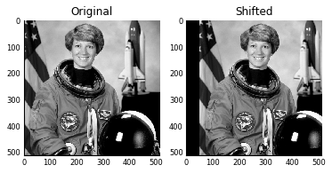
You'll remember our astronaut — Eileen Collins — from chapter 3. We will be shifting this image by 50 pixels to the right then comparing it back to the original until we find the shift that best matches. Obviously this is a silly thing to do, as we know the original position, but this way we know the truth, and we can check how our algorithm is doing. Here's the original and shifted image.
from skimage import data, color
from scipy import ndimage as ndi

astronaut = color.rgb2gray(data.astronaut())
shifted = ndi.shift(astronaut, (0, 50))

fig, axes = plt.subplots(nrows=1, ncols=2)
axes[0].imshow(astronaut)
axes[0].set_title('Original')
axes[1].imshow(shifted)
axes[1].set_title('Shifted');
For the optimization algorithm to do its work, we need some way of defining "dissimilarity"—i.e., the cost function. The easiest way to do this is to simply calculate the average of the squared differences, often called the mean squared error, or MSE.
import numpy as np

def mse(arr1, arr2):
    """Compute the mean squared error between two arrays."""
    return np.mean((arr1 - arr2)**2)
This will return 0 when the images are perfectly aligned, and a higher value otherwise. With this cost function, we can check whether two images are aligned:
ncol = astronaut.shape[1]

# Cover a distance of 90% of the length in columns,
# with one value per percentage point
shifts = np.linspace(-0.9 * ncol, 0.9 * ncol, 181)
mse_costs = []

for shift in shifts:
    shifted_back = ndi.shift(shifted, (0, shift))
    mse_costs.append(mse(astronaut, shifted_back))

fig, ax = plt.subplots()
ax.plot(shifts, mse_costs)
ax.set_xlabel('Shift')
ax.set_ylabel('MSE');
With the cost function defined, we can ask scipy.optimize.minimize
to search for optimal parameters:
from scipy import optimize

def astronaut_shift_error(shift, image):
    corrected = ndi.shift(image, (0, shift))
    return mse(astronaut, corrected)

res = optimize.minimize(astronaut_shift_error, 0, args=(shifted,),
                        method='Powell')

print(f'The optimal shift for correction is: {res.x}')
It worked! We shifted it by +50 pixels, and, thanks to our MSE measure, SciPy's
optimize.minimize function has given us the correct amount of shift (-50) to
get it back to its original state.
It turns out, however, that this was a particularly easy optimization problem, which brings us to the principal difficulty of this kind of alignment: sometimes, the MSE has to get worse before it gets better.
Let's look again at shifting images, starting with the unmodified image:
ncol = astronaut.shape[1]

# Cover a distance of 90% of the length in columns,
# with one value per percentage point
shifts = np.linspace(-0.9 * ncol, 0.9 * ncol, 181)
mse_costs = []

for shift in shifts:
    shifted1 = ndi.shift(astronaut, (0, shift))
    mse_costs.append(mse(astronaut, shifted1))

fig, ax = plt.subplots()
ax.plot(shifts, mse_costs)
ax.set_xlabel('Shift')
ax.set_ylabel('MSE');
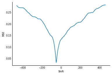
Starting at zero shift, have a look at the MSE value as the shift becomes
increasingly negative: it increases consistently until around -300
pixels of shift, where it starts to decrease again! Only slightly, but it
decreases nonetheless. The MSE bottoms out at around -400, before it
increases again. This is called a local minimum.
Because optimization methods only have access to "nearby"
values of the cost function, if the function improves by moving in the "wrong"
direction, the minimize process will move that way regardless. So, if we
start by an image shifted by -340 pixels:
shifted2 = ndi.shift(astronaut, (0, -340))
minimize will shift it by a further 40 pixels or so,
instead of recovering the original image:
res = optimize.minimize(astronaut_shift_error, 0, args=(shifted2,),
                        method='Powell')

print(f'The optimal shift for correction is {res.x}')
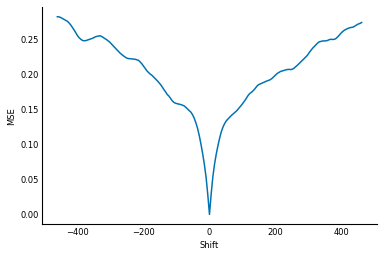
The common solution to this problem is to smooth or downscale the images, which has the dual result of smoothing the objective function. Have a look at the same plot, after having smoothed the images with a Gaussian filter:
from skimage import filters

astronaut_smooth = filters.gaussian(astronaut, sigma=20)

mse_costs_smooth = []
shifts = np.linspace(-0.9 * ncol, 0.9 * ncol, 181)
for shift in shifts:
    shifted3 = ndi.shift(astronaut_smooth, (0, shift))
    mse_costs_smooth.append(mse(astronaut_smooth, shifted3))

fig, ax = plt.subplots()
ax.plot(shifts, mse_costs, label='original')
ax.plot(shifts, mse_costs_smooth, label='smoothed')
ax.legend(loc='lower right')
ax.set_xlabel('Shift')
ax.set_ylabel('MSE');
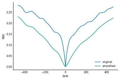
As you can see, with some rather extreme smoothing, the "funnel" of the error function becomes wider, and less bumpy. Rather than smoothing the function itself we can get a similar effect by blurring the images before comparing them. Therefore, modern alignment software uses what's called a Gaussian pyramid, which is a set of progressively lower resolution versions of the same image. We align the the lower resolution (blurrier) images first, to get an approximate alignment, and then progressively refine the alignment with sharper images.
def downsample2x(image):
    offsets = [((s + 1) % 2) / 2 for s in image.shape]
    slices = [slice(offset, end, 2)
              for offset, end in zip(offsets, image.shape)]
    coords = np.mgrid[slices]
    return ndi.map_coordinates(image, coords, order=1)


def gaussian_pyramid(image, levels=6):
    """Make a Gaussian image pyramid.

    Parameters
    ----------
    image : array of float
        The input image.
    max_layer : int, optional
        The number of levels in the pyramid.

    Returns
    -------
    pyramid : iterator of array of float
        An iterator of Gaussian pyramid levels, starting with the top
        (lowest resolution) level.
    """
    pyramid = [image]

    for level in range(levels - 1):
        blurred = ndi.gaussian_filter(image, sigma=2/3)
        image = downsample2x(image)
        pyramid.append(image)

    return reversed(pyramid)
Let's see how the 1D alignment looks along that pyramid:
shifts = np.linspace(-0.9 * ncol, 0.9 * ncol, 181)
nlevels = 8
costs = np.empty((nlevels, len(shifts)), dtype=float)
astronaut_pyramid = list(gaussian_pyramid(astronaut, levels=nlevels))
for col, shift in enumerate(shifts):
    shifted = ndi.shift(astronaut, (0, shift))
    shifted_pyramid = gaussian_pyramid(shifted, levels=nlevels)
    for row, image in enumerate(shifted_pyramid):
        costs[row, col] = mse(astronaut_pyramid[row], image)

fig, ax = plt.subplots()
for level, cost in enumerate(costs):
    ax.plot(shifts, cost, label='Level %d' % (nlevels - level))
ax.legend(loc='lower right', frameon=True, framealpha=0.9)
ax.set_xlabel('Shift')
ax.set_ylabel('MSE');
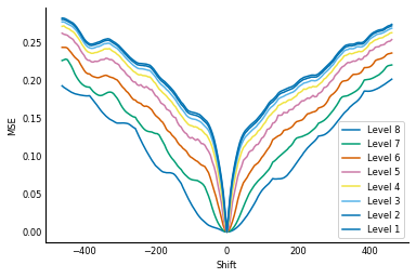
As you can see, at the highest level of the pyramid, that bump at a shift of about -325 disappears. We can therefore get an approximate alignment at that level, then pop down to the lower levels to refine that alignment.
Image registration with optimize
Let's automate that, and try with a "real" alignment, with three parameters: rotation, translation in the row dimension, and translation in the column dimension. This is called a "rigid registration" because there are no deformations of any kind (scaling, skew, or other stretching). The object is considered solid and moved around (including rotation) until a match is found.
To simplify the code, we'll use the scikit-image transform module to compute
the shift and rotation of the image. SciPy's optimize requires a vector of
parameters as input. We first make a
function that will take such a vector and produce a rigid transformation with
the right parameters:
from skimage import transform
def make_rigid_transform(param):
r, tc, tr = param
return transform.SimilarityTransform(rotation=r,
translation=(tc, tr))
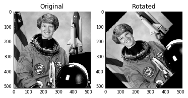
rotated = transform.rotate(astronaut, 45)
fig, axes = plt.subplots(nrows=1, ncols=2)
axes[0].imshow(astronaut)
axes[0].set_title('Original')
axes[1].imshow(rotated)
axes[1].set_title('Rotated');
Next, we need a cost function. This is just MSE, but SciPy requires a specific
format: the first argument needs to be the parameter vector, which it is
optimizing. Subsequent arguments can be passed through the args keyword as a
tuple, but must remain fixed: only the parameter vector can be optimized. In
our case, this is just the rotation angle and the two translation parameters:
def cost_mse(param, reference_image, target_image):
    transformation = make_rigid_transform(param)
    transformed = transform.warp(target_image, transformation, order=3)
    return mse(reference_image, transformed)
Finally, we write our alignment function, which optimizes our cost function at each level of the Gaussian pyramid, using the result of the previous level as a starting point for the next one:
def align(reference, target, cost=cost_mse):
    nlevels = 7
    pyramid_ref = gaussian_pyramid(reference, levels=nlevels)
    pyramid_tgt = gaussian_pyramid(target, levels=nlevels)

    levels = range(nlevels, 0, -1)
    image_pairs = zip(pyramid_ref, pyramid_tgt)

    p = np.zeros(3)

    for n, (ref, tgt) in zip(levels, image_pairs):
        p[1:] *= 2

        res = optimize.minimize(cost, p, args=(ref, tgt), method='Powell')
        p = res.x

        # print current level, overwriting each time (like a progress bar)
        print(f'Level: {n}, Angle: {np.rad2deg(res.x[0]) :.3}, '
              f'Offset: ({res.x[1] * 2**n :.3}, {res.x[2] * 2**n :.3}), '
              f'Cost: {res.fun :.3}', end='\r')

    print('')  # newline when alignment complete
    return make_rigid_transform(p)
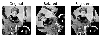
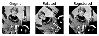
Let's try it with our astronaut image. We rotate it by 60 degrees and add some noise to it. Can SciPy recover the correct transform?
from skimage import util

theta = 60
rotated = transform.rotate(astronaut, theta)
rotated = util.random_noise(rotated, mode='gaussian',
                            seed=0, mean=0, var=1e-3)

tf = align(astronaut, rotated)
corrected = transform.warp(rotated, tf, order=3)

f, (ax0, ax1, ax2) = plt.subplots(1, 3)
ax0.imshow(astronaut)
ax0.set_title('Original')
ax1.imshow(rotated)
ax1.set_title('Rotated')
ax2.imshow(corrected)
ax2.set_title('Registered')
for ax in (ax0, ax1, ax2):
    ax.axis('off')
We're feeling pretty good now. But our choice of parameters actually masked the difficulty of optimization: Let's see what happens with a rotation of 50 degrees, which is closer to the original image:
theta = 50
rotated = transform.rotate(astronaut, theta)
rotated = util.random_noise(rotated, mode='gaussian',
                            seed=0, mean=0, var=1e-3)

tf = align(astronaut, rotated)
corrected = transform.warp(rotated, tf, order=3)

f, (ax0, ax1, ax2) = plt.subplots(1, 3)
ax0.imshow(astronaut)
ax0.set_title('Original')
ax1.imshow(rotated)
ax1.set_title('Rotated')
ax2.imshow(corrected)
ax2.set_title('Registered')
for ax in (ax0, ax1, ax2):
    ax.axis('off')
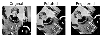
Even though we started closer to the original image, we failed to recover the correct rotation. This is because optimization techniques can get stuck in local minima, little bumps on the road to success, as we saw above with the shift-only alignment. They can therefore be quite sensitive to the starting parameters.
Avoiding local minima with basin hopping
A 1997 algorithm devised by David Wales and Jonathan Doyle 1, called basin-hopping, attempts to avoid local minima by trying an optimization from some initial parameters, then moving away from the found local minimum in a random direction, and optimizing again. By choosing an appropriate step size for these random moves, the algorithm can avoid falling into the same local minimum twice, and thus explore a much larger area of the parameter space than simple gradient-based optimization methods.
We leave it as an exercise to incorporate SciPy's implementation of basin-hopping into our alignment function. You'll need it for later parts of the chapter, so feel free to peek at the solution at the end of the book if you're stuck.
Exercise: Try modifying the align function to use
scipy.optimize.basinhopping, which has explicit strategies to avoid local minima.
Hint: limit using basin-hopping to just the top levels of the pyramid, as it is a slower optimization approach, and could take rather long to run at full image resolution.
Solution: We use basin-hopping at the higher levels of the pyramid, but use Powell's method for the lower levels, because basin-hopping is too computationally expensive to run at full resolution:
David J. Wales and Jonathan P.K. Doyle (1997). Global Optimization by Basin-Hopping and the Lowest Energy Structures of Lennard-Jones Clusters Containing up to 110 Atoms. Journal of Physical Chemistry 101(28):5111–5116 DOI: 10.1021/jp970984n↩
def align(reference, target, cost=cost_mse, nlevels=7, method='Powell'):
    pyramid_ref = gaussian_pyramid(reference, levels=nlevels)
    pyramid_tgt = gaussian_pyramid(target, levels=nlevels)

    levels = range(nlevels, 0, -1)
    image_pairs = zip(pyramid_ref, pyramid_tgt)

    p = np.zeros(3)

    for n, (ref, tgt) in zip(levels, image_pairs):
        p[1:] *= 2
        if method.upper() == 'BH':
            res = optimize.basinhopping(cost, p,
                                        minimizer_kwargs={'args': (ref, tgt)})
            if n <= 4:  # avoid basin-hopping in lower levels
                method = 'Powell'
        else:
            res = optimize.minimize(cost, p, args=(ref, tgt), method='Powell')
        p = res.x
        # print current level, overwriting each time (like a progress bar)
        print(f'Level: {n}, Angle: {np.rad2deg(res.x[0]) :.3}, '
              f'Offset: ({res.x[1] * 2**n :.3}, {res.x[2] * 2**n :.3}), '
              f'Cost: {res.fun :.3}', end='\r')

    print('')  # newline when alignment complete
    return make_rigid_transform(p)
Now let's try that alignment:
from skimage import util

theta = 50
rotated = transform.rotate(astronaut, theta)
rotated = util.random_noise(rotated, mode='gaussian',
                            seed=0, mean=0, var=1e-3)

tf = align(astronaut, rotated, nlevels=8, method='BH')
corrected = transform.warp(rotated, tf, order=3)

f, (ax0, ax1, ax2) = plt.subplots(1, 3)
ax0.imshow(astronaut)
ax0.set_title('Original')
ax1.imshow(rotated)
ax1.set_title('Rotated')
ax2.imshow(corrected)
ax2.set_title('Registered')
for ax in (ax0, ax1, ax2):
    ax.axis('off')
Success! Basin-hopping was able to recover the correct alignment, even in the
problematic case in which the minimize function got stuck.
"What is best?": Choosing the right objective function
At this point, we have a working registration approach, which is most excellent. But it turns out that we've only solved the easiest of registration problems: aligning images of the same modality. This means that we expect bright pixels in the reference image to match up to bright pixels in the test image.
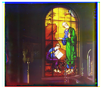
We now move on to aligning different color channels of the same image, where we can no longer rely on the channels having the same modality. This task has historical significance: between 1909 and 1915, the photographer Sergei Mikhailovich Prokudin-Gorskii produced color photographs of the Russian empire before color photography had been invented. He did this by taking three different monochrome pictures of a scene, each with a different color filter placed in front of the lens.
Aligning bright pixels together, as the MSE implicitly does, won't work in this case. Take, for example, these three pictures of a stained glass window in the Church of Saint John the Theologian, taken from the Library of Congress Prokudin-Gorskii Collection:
from skimage import io
stained_glass = io.imread('data/00998v.jpg') / 255  # use float image in [0, 1]
fig, ax = plt.subplots(figsize=(4.8, 7))
ax.imshow(stained_glass)
ax.axis('off');
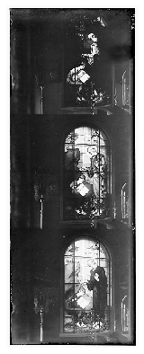
Take a look at St John's robes: they look pitch black in one image, gray in another, and bright white in the third! This would result in a terrible MSE score, even with perfect alignment.
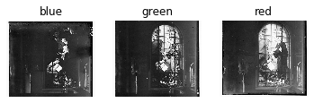
Let's see what we can do with this. We start by splitting the plate into its component channels:
nrows = stained_glass.shape[0]
step = nrows // 3
channels = (stained_glass[:step],
            stained_glass[step:2*step],
            stained_glass[2*step:3*step])
channel_names = ['blue', 'green', 'red']
fig, axes = plt.subplots(1, 3)
for ax, image, name in zip(axes, channels, channel_names):
    ax.imshow(image)
    ax.axis('off')
    ax.set_title(name)
First, we overlay all three images to verify that the alignment indeed needs to be fine-tuned between the three channels:
blue, green, red = channels
original = np.dstack((red, green, blue))
fig, ax = plt.subplots(figsize=(4.8, 4.8), tight_layout=True)
ax.imshow(original)
ax.axis('off');

You can see by the color "halos" around objects in the image that the colors are close to alignment, but not quite. Let's try to align them in the same way that we aligned the astronaut image above, using the MSE. We use one color channel, green, as the reference image, and align the blue and red channels to that.
print('*** Aligning blue to green ***')
tf = align(green, blue)
cblue = transform.warp(blue, tf, order=3)

print('** Aligning red to green ***')
tf = align(green, red)
cred = transform.warp(red, tf, order=3)

corrected = np.dstack((cred, green, cblue))
f, (ax0, ax1) = plt.subplots(1, 2)
ax0.imshow(original)
ax0.set_title('Original')
ax1.imshow(corrected)
ax1.set_title('Corrected')
for ax in (ax0, ax1):
    ax.axis('off')
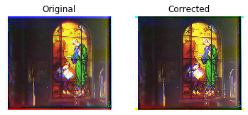
The alignment is a little bit better than with the raw images, because the red and the green channels are correctly aligned, probably thanks to the giant yellow patch of sky. However, the blue channel is still off, because the bright spots of blue don't coincide with the green channel. That means that the MSE will be lower when the channels are mis-aligned so that blue patches overlap with some bright green spots.
We turn instead to a measure called normalized mutual information (NMI), which measures correlations between the different brightness bands of the different images. When the images are perfectly aligned, any object of uniform color will create a large correlation between the shades of the different component channels, and a correspondingly large NMI value. In a sense, NMI measures how easy it would be to predict a pixel value of one image given the value of the corresponding pixel in the other. It was defined in the paper "Studholme, C., Hill, D.L.G., Hawkes, D.J., An Overlap Invariant Entropy Measure of 3D Medical Image Alignment, Patt. Rec. 32, 71–86 (1999)":
$$I(X, Y) = \frac{H(X) + H(Y)}{H(X, Y)},$$where $H(X)$ is the entropy of $X$, and $H(X, Y)$ is the joint entropy of $X$ and $Y$. The numerator describes the entropy of the two images, seen separately, and the denominator the total entropy if they are observed together. Values can vary between 1 (maximally aligned) and 2 (minimally aligned)1. See Chapter 5 for a more in-depth discussion of entropy.
In Python code, this becomes:
A quick handwavy explanation is that entropy is calculated from the histogram of the quantity under consideration. If $X = Y$, then the joint histogram $(X, Y)$ is diagonal, and that diagonal is the same as that of either $X$ or $Y$. Thus, $H(X) = H(Y) = H(X, Y)$ and $I(X, Y) = 2$.↩
from scipy.stats import entropy

def normalized_mutual_information(A, B):
    """Compute the normalized mutual information.

    The normalized mutual information is given by:

                H(A) + H(B)
      Y(A, B) = -----------
                  H(A, B)

    where H(X) is the entropy ``- sum(x log x) for x in X``.

    Parameters
    ----------
    A, B : ndarray
        Images to be registered.

    Returns
    -------
    nmi : float
        The normalized mutual information between the two arrays, computed at a
        granularity of 100 bins per axis (10,000 bins total).
    """
    hist, bin_edges = np.histogramdd([np.ravel(A), np.ravel(B)], bins=100)
    hist /= np.sum(hist)

    H_A = entropy(np.sum(hist, axis=0))
    H_B = entropy(np.sum(hist, axis=1))
    H_AB = entropy(np.ravel(hist))

    return (H_A + H_B) / H_AB
Now we define a cost function to optimize, as we defined cost_mse above:
def cost_nmi(param, reference_image, target_image):
    transformation = make_rigid_transform(param)
    transformed = transform.warp(target_image, transformation, order=3)
    return -normalized_mutual_information(reference_image, transformed)
Finally, we use this with our basinhopping-optimizing aligner:
print('*** Aligning blue to green ***')
tf = align(green, blue, cost=cost_nmi)
cblue = transform.warp(blue, tf, order=3)

print('** Aligning red to green ***')
tf = align(green, red, cost=cost_nmi)
cred = transform.warp(red, tf, order=3)

corrected = np.dstack((cred, green, cblue))
fig, ax = plt.subplots(figsize=(4.8, 4.8), tight_layout=True)
ax.imshow(corrected)
ax.axis('off')
What a glorious image! Realize that this artifact was created before color photography existed! Notice God's pearly white robes, John's white beard, and the white pages of the book held by Prochorus, his scribe — all of which were missing from the MSE-based alignment, but look wonderfully clear using NMI. Notice also the realistic gold of the candlesticks in the foreground.
We've illustrated the two key concepts in function optimization in this chapter: understanding local minima and how to avoid them, and choosing the right function to optimize to achieve a particular objective. Solving these allows you to apply optimization to a wide array of scientific problems!