Linear algebra in SciPy

No one can be told what the matrix is. You have to see it for yourself.

— Morpheus, The Matrix

Just like Chapter 4, which dealt with the Fast Fourier Transform, this chapter will feature an elegant method. We want to highlight the packages available in SciPy to do linear algebra, which forms the basis of much scientific computing.

Linear algebra basics

A chapter in a programming book is not really the right place to learn about linear algebra itself, so we assume familiarity with linear algebra concepts. At a minimum, you should know that linear algebra involves vectors (ordered collections of numbers) and their transformations by multiplying them with matrices (collections of vectors). If all of this sounded like gibberish to you, you should probably pick up an introductory linear algebra textbook before reading this. We highly recommend Gil Strang's Linear Algebra and its Applications. Introductory is all you need though — we hope to convey the power of linear algebra while keeping the operations relatively simple!

As an aside, we will break Python notation convention in order to match linear algebra conventions: in Python, variables names should usually begin with a lower case letter. However, in linear algebra, matrices are denoted by a capital letter, while vectors and scalar values are lowercase. Since we're going to be dealing with quite a few matrices and vectors, following the linear algebra convention helps to keep them straight. Therefore, variables that represent matrices will start with a capital letter, while vectors and numbers will start with lowercase:

In mathematical notation, the vectors would typically be written in boldface, as in $\mathbf{v}$ and $\mathbf{w}$, while the scalars would not, as in $m$ and $n$. In Python code, we can't make that distinction, so we will rely instead on context to keep scalars and vectors straight.

Laplacian matrix of a graph

We discussed graphs in chapter 3, where we represented image regions as nodes, connected by edges between them. But we used a rather simple method of analysis: we thresholded the graph, removing all edges above some value. Thresholding works in simple cases, but can easily fail, because all you need is one value to fall on the wrong side of the threshold for the approach to fail.

As an example, suppose you are at war, and your enemy is camped just across the river from your forces. You want to cut them off, so you decide to blow up all the bridges between you. Intelligence suggests that you need $t$ kilograms of TNT to blow each bridge crossing the river, but the bridges in your own territory can withstand $t+1$ kg. You might, having just read chapter 3 of Elegant SciPy, order your commandos to detonate $t$ kg of TNT on every bridge in the region. But, if intelligence was wrong about just one bridge crossing the river, and it remains standing, the enemy's army can come marching through! Disaster!

So, in this chapter, we will explore some alternative approaches to graph analysis, based on linear algebra. It turns out that we can think of a graph, $G$, as an adjacency matrix, in which we number the nodes of the graph from $0$ to $n-1$, and place a 1 in row $i$, column $j$ of the matrix whenever there is an edge from node $i$ to node $j$. In other words, if we call the adjacency matrix $A$, then $A_{i, j} = 1$ if and only if the edge $(i, j)$ is in $G$. We can then use linear algebra techniques to study this matrix, often with striking results.

The degree of a node is defined as the number of edges touching it. For example, if a node is connected to five other nodes in a graph, its degree is 5. (Later, we will differentiate between out-degree and in-degree, when edges have a "from" and "to".) In matrix terms, the degree corresponds to the sum of the values in a row or column.

The Laplacian matrix of a graph (just "the Laplacian" for short) is defined as the degree matrix, $D$, which contains the degree of each node along the diagonal and zero everywhere else, minus the adjacency matrix $A$:

$ L = D - A $

We definitely can't fit all of the linear algebra theory needed to understand the properties of this matrix, but suffice it to say: it has some great properties. We will exploit a couple in the following paragraphs.

First, we will look at the eigenvectors of $L$. An eigenvector $v$ of a matrix $M$ is a vector that satisfies the property $Mv = \lambda v$ for some number $\lambda$, known as the eigenvalue. In other words, $v$ is a special vector in relation to $M$ because $Mv$ simply changes the size of the vector, without changing its direction. As we will soon see, eigenvectors have many useful properties — sometimes seeming even magical!

As an example, a 3x3 rotation matrix $R$, when multiplied by any 3-dimensional vector $p$, rotates it $30^\circ$ degrees around the z-axis. $R$ will rotate all vectors except for those that lie on the z-axis. For those, we'll see no effect, or $Rp = p$, i.e. $Rp = \lambda p$ with eigenvalue $\lambda = 1$.

Exercise: Consider the rotation matrix

$ R = \begin{bmatrix} \cos \theta & -\sin \theta & 0 \\ \sin \theta & \cos \theta & 0\\ 0 & 0 & 1\\ \end{bmatrix} $

When $R$ is multiplied with a 3-dimensional column-vector $p = \left[ x\, y\, z \right]^T$, the resulting vector $R p$ is rotated by $\theta$ degrees around the z-axis.

1. For $\theta = 45^\circ$, verify (by testing on a few arbitrary vectors) that $R$ rotates these vectors around the z axis. Remember that matrix multiplication in Python is denoted with @.

2. What does the matrix $S = RR$ do? Verify this in Python.

3. Verify that multiplying by $R$ leaves the vector $\left[ 0\, 0\, 1\right]^T$ unchanged. In other words, $R p = 1 p$, which means $p$ is an eigenvector of $R$ with eigenvalue 1.

4. Use np.linalg.eig to find the eigenvalues and eigenvectors of $R$, and verify that $\left[0, 0, 1\right]^T$ is indeed among them, and that it corresponds to the eigenvalue 1.

Solution:

Part 1:

Part 2:

Since multiplying a vector by $R$ rotates it 45 degrees, multiplying the result by $R$ again should result in the original vector being rotated 90 degrees. Matrix multiplication is associative, which means that $R(Rv) = (RR)v$, so $S = RR$ should rotate vectors by 90 degrees around the z-axis.

Part 3:

R rotates both the x and y axes, but not the z-axis.

Part 4:

Looking at the documentation of eig, we see that it returns two values: a 1D array of eigenvalues, and a 2D array where each column contains the eigenvector corresponding to each eigenvalue.

In addition to some complex-valued eigenvalues and vectors, we see the value 1 associated with the vector $\left[0, 0, 1\right]^T$.

Back to the Laplacian. A common problem in network analysis is visualization. How do you draw nodes and edges in such a way that you don't get a complete mess such as this one?

One way is to put nodes that share many edges close together. It turns out that this can be done by using the second-smallest eigenvalue of the Laplacian matrix, and its corresponding eigenvector, which is so important it has its own name: the Fiedler vector.

Let's use a minimal network to illustrate this. We start by creating the adjacency matrix:

We can use NetworkX to draw this network. First, we initialize matplotlib as usual:

Now, we can plot it:

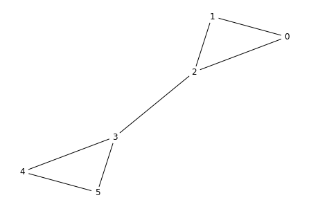
You can see that the nodes fall naturally into two groups, 0, 1, 2 and 3, 4, 5. Can the Fiedler vector tell us this? First, we must compute the degree matrix and the Laplacian. We first get the degrees by summing along either axis of $A$. (Either axis works because $A$ is symmetric.)

We then put those degrees into a diagonal matrix of the same shape as A, the degree matrix. We can use the np.diag function to do this:

Finally, we get the Laplacian from the definition:

Because $L$ is symmetric, we can use the np.linalg.eigh function to compute the eigenvalues and eigenvectors:

You can verify that the values returned satisfy the definition of eigenvalues and eigenvectors. For example, one of the eigenvalues is 3:

And we can check that multiplying the matrix $L$ by the corresponding eigenvector does indeed multiply the vector by 3:

As mentioned above, the Fiedler vector is the vector corresponding to the second-smallest eigenvalue of $L$. Sorting the eigenvalues tells us which one is the second-smallest:

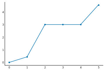
It's the first non-zero eigenvalue, close to 0.4. The Fiedler vector is the corresponding eigenvector:

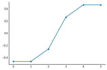
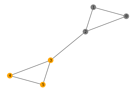
It's pretty remarkable: by looking at the sign of the elements of the Fiedler vector, we can separate the nodes into the two groups we identified in the drawing!

Laplacians with brain data

Let's demonstrate this process in a real-world example by laying out the brain cells in a worm, as shown in Figure 2 from the Varshney et al paper that we introduced in Chapter 3. (Information on how to do this is in the supplementary material for the paper.) To obtain their layout of the worm brain neurons, they used a related matrix, the degree-normalized Laplacian.

Because the order of the neurons is important in this analysis, we will use a preprocessed dataset, rather than clutter this chapter with data cleaning. We got the original data from Lav Varshney's website, and the processed data is in our data/ directory.

First, let's load the data. There are four components:

• the network of chemical synapses, through which a pre-synaptic neuron sends a chemical signal to a post-synaptic neuron,
• the gap junction network, which contains direct electrical contacts between neurons),
• the neuron IDs (names), and
• the three neuron types:
  • sensory neurons, those that detect signals coming from the outside world, encoded as 0;
  • motor neurons, those that activate muscles, enabling the worm to move, encoded as 2; and
  • interneurons, the neurons in between, which enable complex signal processing to occur between sensory neurons and motor neurons, encoded as 1.

We then simplify the network, adding the two kinds of connections together, and removing the directionality of the network by taking the average of in-connections and out-connections of neurons. This seems a bit like cheating but, since we are only looking for the layout of the neurons on a graph, we only care about whether neurons are connected, not in which direction. We are going to call the resulting matrix the connectivity matrix, $C$, which is just a different kind of adjacency matrix.

To get the Laplacian matrix $L$, we need the degree matrix $D$, which contains the degree of node i at position [i, i], and zeros everywhere else.

Now, we can get the Laplacian just like before:

The vertical coordinates in Fig 2 are given by arranging nodes such that, on average, neurons are as close as possible to "just above" their downstream neighbors. Varshney et al call this measure "processing depth," and it's obtained by solving a linear equation involving the Laplacian. We use scipy.linalg.pinv, the pseudoinverse, to solve it:

(Note the use of the @ symbol, which was introduced in Python 3.5 to denote matrix multiplication. As we noted in the preface and in Chapter 5, in previous versions of Python, you would need to use the function np.dot.)

In order to obtain the degree-normalized Laplacian, $Q$, we need the inverse square root of the $D$ matrix:

Finally, we are able to extract the $x$ coordinates of the neurons to ensure that highly-connected neurons remain close: the eigenvector of $Q$ corresponding to its second-smallest eigenvalue, normalized by the degrees:

Note from the documentation of numpy.linalg.eig:

"The eigenvalues are not necessarily ordered."

Although the documentation in SciPy's eig lacks this warning, it remains true in this case. We must therefore sort the eigenvalues and the corresponding eigenvector columns ourselves:

Now we can find the eigenvector we need to compute the affinity coordinates:

(The reasons for using this vector are too long to explain here, but appear in the paper's supplementary material, linked above. The short version is that choosing this vector minimizes the total length of the links between neurons.)

There is one small kink that we must address before proceeding: eigenvectors are only defined up to a multiplicative constant. This follows simply from the definition of an eigenvector: suppose $v$ is an eigenvector of the matrix $M$, with corresponding eigenvalue $\lambda$. Then $\alpha v$ is also an eigenvector of $M$ for any scalar number $\alpha$, because $Mv = \lambda v$ implies $M(\alpha v) = \lambda (\alpha v)$. So, it is arbitrary whether a software package returns $v$ or $-v$ when asked for the eigenvectors of $M$. In order to make sure we reproduce the layout from the Varshney et al. paper, we must make sure that the vector is pointing in the same direction as theirs, rather than the opposite direction. We do this by choosing an arbitrary neuron from their Figure 2, and checking the sign of x at that position. We then reverse it if it doesn't match its sign in Figure 2 of the paper.

Now it's just a matter of drawing the nodes and the edges. We color them according to the type stored in neuron_types, using the appealing and functional "colorblind" colorbrewer palette:

Now, let's use that function to plot the neurons:

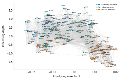
There you are: a worm brain! As discussed in the original paper, you can see the top-down processing from sensory neurons to motor neurons through a network of interneurons. You can also see two distinct groups of motor neurons: these correspond to the neck (left) and body (right) body segments of the worm.

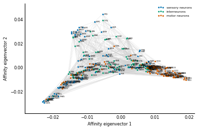
Exercise: How do you modify the above code to show the affinity view in Figure 2B from the paper?

Solution: In the affinity view, instead of using the processing depth on the y-axis, we use the normalized third eigenvector of Q, just like we did with x. (And we invert it if necessary, just like we did with x!)

Challenge: linear algebra with sparse matrices

The above code uses numpy arrays to hold the matrix and perform the necessary computations. Because we are using a small graph of fewer than 300 nodes, this is feasible. However, for larger graphs, it would fail.

For example, one might want to analyse the relationships between libraries listed on the Python Package Index, or PyPI, which contains over one hundred thousand packages. Holding the Laplacian matrix for this graph would take up $8 \left(100 \times 10^3\right)^2 = 8 \times 10^10$ bytes, or 80GB, of RAM. If you add to that the adjacency, symmetric adjacency, pseudoinverse, and, say, two temporary matrices used during calculations, you climb up to 480GB, beyond the reach of most desktop computers.

"Ha!", some of you might be thinking. "Ha! My desktop has 512GB of RAM! It would make short work of this so-called 'large' graph!"

Perhaps. But you might also want to analyze the Association for Computing Machinery (ACM) citation graph, a network of over two million scholarly works and references. That Laplacian would take up 32 terabytes of RAM.

However, we know that the dependency and reference graphs are sparse: packages usually depend on just a few other packages, not on the whole of PyPI. And papers and books usually only reference a few others, too. So we can hold the above matrices using the sparse data structures from scipy.sparse (see Chapter 5), and use the linear algebra functions in scipy.sparse.linalg to compute the values we need.

Try to explore the documentation in scipy.sparse.linalg to come up with a sparse version of the above computation.

Hint: the pseudoinverse of a sparse matrix is, in general, not sparse, so you can't use it here. Similarly, you can't get all the eigenvectors of a sparse matrix, because they would together make up a dense matrix.

You'll find parts of the solution below (and of course in the solutions chapter), but we highly recommend that you try it out on your own.

Challenge accepted

For the purposes of this challenge, we are going to use the small connectome above, because it's easier to visualise what is going on. In later parts of the challenge we'll use these techniques to analyze larger networks.

First, we start with the adjacency matrix, A, in a sparse matrix format, in this case, CSR, which is the most common format for linear algebra. We'll append s to the names of all the matrices to indicate that they are sparse.

We can create our connectivity matrix in the same way:

In order to get the degrees matrix, we can use the "diags" sparse format, which stores diagonal and off-diagonal matrices.

Getting the Laplacian is straightforward:

Now we want to get the processing depth. Remember that getting the pseudo-inverse of the Laplacian matrix is out of the question, because it will be a dense matrix (the inverse of a sparse matrix is not generally sparse itself). However, we were actually using the pseudo-inverse to compute a vector $z$ that would satisfy $L z = b$, where $b = C \odot \textrm{sign}\left(A - A^T\right) \mathbf{1}$. (You can see this in the supplementary material for Varshney et al.) With dense matrices, we can simply use $z = L^+b$. With sparse ones, though, we can use one of the solvers (see sidebox, "Solvers") in sparse.linalg.isolve to get the z vector after providing L and b, no inversion required!

Finally, we must find the eigenvectors of $Q$, the degree-normalized Laplacian, corresponding to its second and third smallest eigenvalues.

You might recall from Chapter 5 that the numerical data in sparse matrices is in the .data attribute. We use that to invert the degrees matrix:

Finally, we use SciPy's sparse linear algebra functions to find the desired eigenvectors. The $Q$ matrix is symmetric, so we can use the eigsh function, specialized for symmetric matrices, to compute them. We use the which keyword argument to specify that we want the eigenvectors corresponding to the smallest eigenvalues, and k to specify that we need the 3 smallest:

Finally, we normalize the eigenvectors to get the x and y coordinates (and flip these if necessary):

(Note that the eigenvector corresponding to the smallest eigenvalue is always a vector of all ones, which we're not interested in.) We can now reproduce the above plots!

Solvers {.callout}

SciPy has several sparse iterative solvers available, and it is not always obvious which to use. Unfortunately, that question also has no easy answer: different algorithms have different strengths in terms of speed of convergence, stability, accuracy, and memory use (amongst others). It is also not possible to predict, by looking at the input data, which algorithm will perform best.

Here is a rough guideline for choosing an iterative solver:

• If A, the input matrix, is symmetric and positive definite, use the Conjugate Gradient solver cg. If A is symmetric, but near-singular or indefinite, try the Minimum Residual iteration method minres.

• For non-symmetric systems, try the Biconjugate Gradient Stabilized method, bicgstab. The Conjugate Gradient Squared method, cgs, is a bit faster, but has more erratic convergence.

• If you need to solve many similar systems, use the LGMRES algorithm lgmres.

• If A is not square, use the least squares algorithm lsmr.

For further reading, see

• How Fast are Nonsymmetric Matrix Iterations?, Noël M. Nachtigal, Satish C. Reddy, and Lloyd N. Trefethen SIAM Journal on Matrix Analysis and Applications 1992 13:3, 778-795.

• Survey of recent Krylov methods, Jack Dongarra, http://www.netlib.org/linalg/html_templates/node50.html

PageRank: linear algebra for reputation and importance

Another application of linear algebra and eigenvectors is Google's PageRank algorithm, which is punnily named both for webpages and for one of its co-founders, Larry Page.

To rank webpages by importance, you might count how many other webpages link to it. After all, if everyone is linking to a particular page, it must be good, right? But this metric is easily gamed: to make your own webpage rise in the rankings, just create as many other webpages as you can and have them all link to your original page.

The key insight that drove Google's early success was that important webpages are not linked to by just many webpages, but by important webpages. And how do we know that those other pages are important? Because they themselves are linked to by important pages. And so on.

This recursive definition implies that page importance can be measured by an eigenvector of the so-called transition matrix, which contains the links between webpages. Suppose you have your vector of importance $\boldsymbol{r}$, and your matrix of links $M$. You don't know $\boldsymbol{r}$ yet, but you do know that the importance of a page is proportional to the sum of importances of the pages that link to it: $\boldsymbol{r} = \alpha M \boldsymbol{r}$, or $M \boldsymbol{r} = \lambda \boldsymbol{r}$, for $\lambda = 1/\alpha$. That's just the definition of an eigenvalue!

By ensuring some special properties are satisfied by the transition matrix, we can further determine that the required eigenvalue is 1, and that it is the largest eigenvalue of $M$.

The transition matrix imagines a web surfer, often named Webster, randomly clicking a link from each webpage he visits, and then asks, what's the probability that he ends up at any given page? This probability is called the PageRank.

Since Google's rise, researchers have been applying PageRank to all sorts of networks. We'll use an example by Stefano Allesina and Mercedes Pascual, which they published in PLoS Computational Biology. They thought to apply the method in ecological food webs, networks that link species to those that they eat.

Naively, if you wanted to see how critical a species was for an ecosystem, you would look at how many species eat it. If it's many, and that species disappeared, then all its "dependent" species might disappear with it. In network parlance, you could say that its in-degree determines its ecological importance.

Could PageRank be a better measure of importance for an ecosystem?

Professor Allesina kindly provided us with a few food webs to play around with. We've saved one of these, from the St Marks National Wildlife Refuge in Florida, in the Graph Markup Language format. The web was described in 1999 by Robert R. Christian and Joseph J. Luczovich. In the dataset, a node $i$ has an edge to node $j$ if species $i$ eats species $j$.

We'll start by loading in the data, which NetworkX knows how to read trivially:

Next, we get the sparse matrix corresponding to the graph. Because a matrix only holds numerical information, we need to maintain a separate list of package names corresponding to the matrix rows/columns:

From the adjacency matrix, we can derive a transition probability matrix, where every edge is replaced by a probability of 1 over the number of outgoing edges from that species. In the food web, it might make more sense to call this a lunch probability matrix.

The total number of species in our matrix is going to be used a lot, so let's call it $n$:

Next, we need the degrees, and, in particular, the diagonal matrix containing the inverse of the out-degrees of each node on the diagonal:

Normally, the PageRank score would simply be the first eigenvector of the transition matrix. If we call the transition matrix $M$ and the vector of PageRank values $r$, we have:

$$ \boldsymbol{r} = M\boldsymbol{r} $$

But the np.seterr call above is a clue that it's not quite so simple. The PageRank approach only works when the transition matrix is a column-stochastic matrix, in which every column sums to 1. Additionally, every page must be reachable from every other page, even if the path to reach it is very long.

In our food web, this causes problems, because the bottom of the food chain, what the authors call detritus (basically sea sludge), doesn't actually eat anything (the Circle of Life notwithstanding), so you can't reach other species from it.

Young Simba: But, Dad, don't we eat the antelope?

Mufasa: Yes, Simba, but let me explain. When we die, our bodies become the grass, and the antelope eat the grass. And so we are all connected in the great Circle of Life.

— The Lion King

To deal with this, the PageRank algorithm uses a so-called "damping factor", usually taken to be 0.85. This means that 85% of the time, the algorithm follows a link at random, but for the other 15%, it randomly jumps to any arbitrary page. It's as if every page had a low probability link to every other page. Or, in our case, it's as if shrimp, on rare occasions, ate sharks. It might seem non-sensical but bear with us! It is, in fact, the mathematical representation of the Circle of Life. We'll set it to 0.85, but actually it doesn't really matter for this analysis: the results are similar for a large range of possible damping factors.

If we call the damping factor $d$, then the modified PageRank equation is:

$$ \boldsymbol{r} = dM\boldsymbol{r} + \frac{1-d}{n} \boldsymbol{1} $$

and

$$ (\boldsymbol{I} - dM)\boldsymbol{r} = \frac{1-d}{n} \boldsymbol{1} $$

We can solve this equation using scipy.sparse.linalg's direct solver, spsolve. Depending on the structure and size of a linear algebra problem, though, it might be more efficient to use an iterative solver. See the scipy.sparse.linalg documentation for more information on this.

We now have the "foodrank" of the St. Marks food web!

So how does a species' foodrank compare to the number of other species eating it?

We now draw the plot. Having explored the dataset before writing this, we have pre-labeled some interesting nodes in the plot:

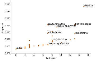
Sea sludge ("detritus") is the most important element both by number of species feeding on it (15) and by PageRank (>0.003). But the second most important element is not benthic algae, which feeds 13 other species, but rather phytoplankton, which feeds just 7! That's because other important species feed on it. On the bottom left, we've got sea gulls, who, we can now confirm, do bugger-all for the ecosystem. Those vicious predatory shrimps (we're not making this up) support the same number of species as phytoplankton, but they are less essential species, so they end up with a lower foodrank.

Although we won't do it here, Allesina and Pascual go on to model the ecological impact of species extinction, and indeed find that PageRank predicts ecological importance better than in-degree.

Before we wrap up though, we'll note that PageRank can be computed several different ways. One way, complementary to what we did above, is called the power method, and it's quite, well, powerful! It stems from the Perron-Frobenius theorem, which states, among other things, that a stochastic matrix has 1 as an eigenvalue, and that this is its largest eigenvalue. (The corresponding eigenvector is the PageRank vector.) What this means is that, whenever we multiply any vector by $M$, its component pointing towards this major eigenvector stays the same, while all other components shrink by a multiplicative factor. The consequence is that if we multiply some random starting vector by $M$ repeatedly, we should eventually get the PageRank vector!

SciPy makes this very efficient with its sparse matrix module:

Exercise: In the above iteration, note that Trans is not column-stochastic, so the $r$ vector gets shrunk at each iteration. In order to make the matrix stochastic, we have to replace every zero-column by a column of all $1/n$. This is too expensive, but computing the iteration is cheaper. How can you modify the code above to ensure that $r$ remains a probability vector throughout?

Solution: In order to have a stochastic matrix, all columns of the transition matrix must sum to 1. This is not satisfied when a species isn't eaten by any others: that column will consist of all zeroes. Replacing all those columns by $1/n \boldsymbol{1}$, however, would be expensive.

The key is to realise that every row will contribute the same amount to the multiplication of the transition matrix by the current probability vector. That is to say, adding these columns will add a single value to the result of the iteration multiplication. What value? $1/n$ times the elements of $r$ that correspond to a dangling node. This can be expressed as a dot-product of a vector containing $1/n$ for positions corresponding to dangling nodes, and zero elswhere, with the vector $r$ for the current iteration.

Try this out manually for a few iterations. Notice that if you start with a stochastic vector (a vector whose elements all sum to 1), the next vector will still be a stochastic vector. Thus, the output PageRank from this function will be a true probability vector, and the values will represent the probability that we end up at a particular species when following links in the food chain.

Exercise: Verify that these three methods all give the same ranking for the nodes. numpy.corrcoef might be a useful function for this.

Solution: np.corrcoef gives the Pearson correlation coefficient between all pairs of a list of vectors. This coefficient will be equal to 1 if and only if two vectors are scalar multiples of each other. Therefore, a correlation coefficient of 1 is sufficient to show that the above methods produce the same ranking.

Concluding remarks

The field of linear algebra is far too broad to adequately cover in a chapter, but this chapter gave you a glimpse into its power, and of the way Python, NumPy, and SciPy make its elegant algorithms accessible.